Machine vision capability for Python.

Project description


Machine Vision Toolbox for Python
 |
A Python implementation of the Machine Vision Toolbox for MATLAB® |
Synopsis
The Machine Vision Toolbox for Python (MVTB-P) provides many functions that are useful in machine vision and vision-based control. It is a somewhat eclectic collection reflecting my personal interest in areas of photometry, photogrammetry, colorimetry. It includes over 100 functions spanning operations such as image file reading and writing, acquisition, display, filtering, blob, point and line feature extraction, mathematical morphology, homographies, visual Jacobians, camera calibration and color space conversion. With input from a web camera and output to a robot (not provided) it would be possible to implement a visual servo system entirely in Python.
An image is usually treated as a rectangular array of scalar values representing intensity or perhaps range, or 3-vector values representing a color image. The matrix is the natural datatype of NumPy and thus makes the manipulation of images easily expressible in terms of arithmetic statements in Python.
Advantages of this Python Toolbox are that:
- it uses, as much as possibe, OpenCV, which is a portable, efficient, comprehensive and mature collection of functions for image processing and feature extraction;
- it wraps the OpenCV functions in a consistent way, hiding some of the complexity of OpenCV;
- it is has similarity to the Machine Vision Toolbox for MATLAB.
Getting going
Using pip
Install a snapshot from PyPI
% pip install machinevision-toolbox-python
From GitHub
Install the current code base from GitHub and pip install a link to that cloned copy
% git clone https://github.com/petercorke/machinevision-toolbox-python.git
% cd machinevision-toolbox-python
% pip install -e .
Examples
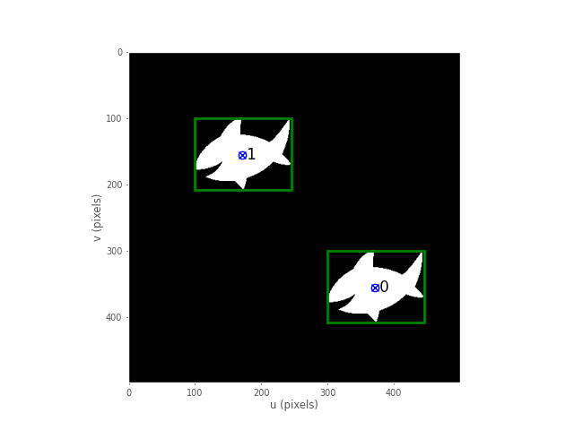
Binary blobs
import machinevisiontoolbox as mvtb
import matplotlib.pyplot as plt
im = mvtb.Image('shark2.png')   # read a binary image of two sharks
fig = im.disp();   # display it with interactive viewing tool
f = im.blobs()  # find all the white blobs
print(f)

	┌───┬────────┬──────────────┬──────────┬───────┬───────┬─────────────┬────────┬────────┐
	│id │ parent │     centroid │     area │ touch │ perim │ circularity │ orient │ aspect │
	├───┼────────┼──────────────┼──────────┼───────┼───────┼─────────────┼────────┼────────┤
	│ 0 │     -1 │ 371.2, 355.2 │ 7.59e+03 │ False │ 557.6 │       0.341 │  82.9° │  0.976 │
	│ 1 │     -1 │ 171.2, 155.2 │ 7.59e+03 │ False │ 557.6 │       0.341 │  82.9° │  0.976 │
	└───┴────────┴──────────────┴──────────┴───────┴───────┴─────────────┴────────┴────────┘

f.plot_box(fig, color='g')  # put a green bounding box on each blob
f.plot_centroid(fig, 'o', color='y')  # put a circle+cross on the centroid of each blob
f.plot_centroid(fig, 'x', color='y')
plt.show(block=True)  # display the result
Binary blob hierarchy
We can load a binary image with nested objects
im = mvtb.Image('multiblobs.png')
im.disp()
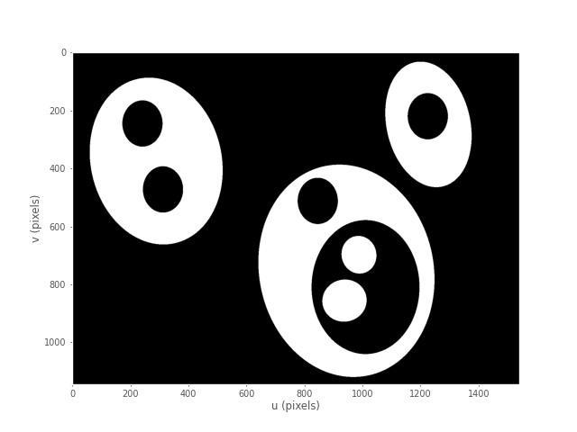
f  = im.blobs()
print(f)
	┌───┬────────┬───────────────┬──────────┬───────┬────────┬─────────────┬────────┬────────┐
	│id │ parent │      centroid │     area │ touch │  perim │ circularity │ orient │ aspect │
	├───┼────────┼───────────────┼──────────┼───────┼────────┼─────────────┼────────┼────────┤
	│ 0 │      1 │  898.8, 725.3 │ 1.65e+05 │ False │ 2220.0 │       0.467 │  86.7° │  0.754 │
	│ 1 │      2 │ 1025.0, 813.7 │ 1.06e+05 │ False │ 1387.9 │       0.769 │ -88.9° │  0.739 │
	│ 2 │     -1 │  938.1, 855.2 │ 1.72e+04 │ False │  490.7 │       1.001 │  88.7° │  0.862 │
	│ 3 │     -1 │  988.1, 697.2 │ 1.21e+04 │ False │  412.5 │       0.994 │ -87.8° │  0.809 │
	│ 4 │     -1 │  846.0, 511.7 │ 1.75e+04 │ False │  496.9 │       0.992 │ -90.0° │  0.778 │
	│ 5 │      6 │  291.7, 377.8 │  1.7e+05 │ False │ 1712.6 │       0.810 │ -85.3° │  0.767 │
	│ 6 │     -1 │  312.7, 472.1 │ 1.75e+04 │ False │  495.5 │       0.997 │ -89.9° │  0.777 │
	│ 7 │     -1 │  241.9, 245.0 │ 1.75e+04 │ False │  496.9 │       0.992 │ -90.0° │  0.777 │
	│ 8 │      9 │ 1228.0, 254.3 │ 8.14e+04 │ False │ 1215.2 │       0.771 │ -77.2° │  0.713 │
	│ 9 │     -1 │ 1225.2, 220.0 │ 1.75e+04 │ False │  496.9 │       0.992 │ -90.0° │  0.777 │
	└───┴────────┴───────────────┴──────────┴───────┴────────┴─────────────┴────────┴────────┘
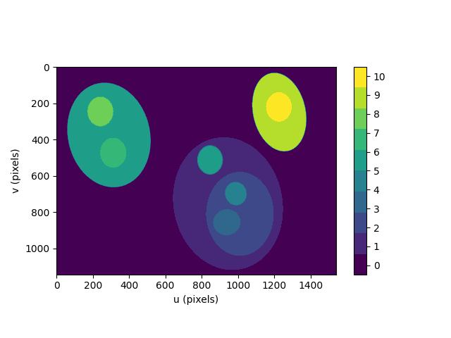
We can display a label image, where the value of each pixel is the label of the blob that the pixel belongs to
out = f.labelImage(im)
out.stats()
out.disp(block=True, colormap='jet', cbar=True, vrange=[0,len(f)-1])
and request the blob label image which we then display
>> [label, m] = ilabel(im);
>> idisp(label, 'colormap', jet, 'bar')
Camera modelling
cam = mvtb.CentralCamera(f=0.015, rho=10e-6, imagesize=[1280, 1024], pp=[640, 512], name='mycamera')
print(cam)
	           Name: mycamera [CentralCamera]
	   focal length: (array([0.015]), array([0.015]))
	     pixel size: 1e-05 x 1e-05
	   principal pt: (640.0, 512.0)
	     image size: 1280.0 x 1024.0
	   focal length: (array([0.015]), array([0.015]))
	           pose: t = 0, 0, 0; rpy/zyx = 0°, 0°, 0°
and its intrinsic parameters are
print(cam.K)
	[[1.50e+03 0.00e+00 6.40e+02]
	 [0.00e+00 1.50e+03 5.12e+02]
	 [0.00e+00 0.00e+00 1.00e+00]]
We can define an arbitrary point in the world
P = [0.3, 0.4, 3.0]
and then project it into the camera
p = cam.project(P)
print(p)
	[790. 712.]
which is the corresponding coordinate in pixels. If we shift the camera slightly the image plane coordinate will also change
p = cam.project(P, T=SE3(0.1, 0, 0) )
print(p)
[740. 712.]
We can define an edge-based cube model and project it into the camera's image plane
X, Y, Z = mkcube(0.2, pose=SE3(0, 0, 1), edge=True)
cam.mesh(X, Y, Z)

Color space
Plot the CIE chromaticity space
showcolorspace('xy')

Load the spectrum of sunlight at the Earth's surface and compute the CIE xy chromaticity coordinates
nm = 1e-9
lam = np.linspace(400, 701, 5) * nm # visible light
sun_at_ground = loadspectrum(lam, 'solar')
xy = lambda2xy(lambda, sun_at_ground)
print(xy)
	[[0.33272798 0.3454013 ]]
print(colorname(xy, 'xy'))
	khaki
Hough transform
im = iread('church.png', 'grey', 'double');
edges = icanny(im);
h = Hough(edges, 'suppress', 10);
lines = h.lines();

idisp(im, 'dark');
lines(1:10).plot('g');

lines = lines.seglength(edges);

lines(1)

k = find( lines.length > 80);

lines(k).plot('b--')

SURF features
We load two images and compute a set of SURF features for each
>> im1 = iread('eiffel2-1.jpg', 'mono', 'double');
>> im2 = iread('eiffel2-2.jpg', 'mono', 'double');
>> sf1 = isurf(im1);
>> sf2 = isurf(im2);
We can match features between images based purely on the similarity of the features, and display the correspondences found
>> m = sf1.match(sf2)
m =
644 corresponding points (listing suppressed)
>> m(1:5)
ans =

(819.56, 358.557) <-> (708.008, 563.342), dist=0.002137
(1028.3, 231.748) <-> (880.14, 461.094), dist=0.004057
(1027.6, 571.118) <-> (885.147, 742.088), dist=0.004297
(927.724, 509.93) <-> (800.833, 692.564), dist=0.004371
(854.35, 401.633) <-> (737.504, 602.187), dist=0.004417
>> idisp({im1, im2})
>> m.subset(100).plot('w')

Clearly there are some bad matches here, but we we can use RANSAC and the epipolar constraint implied by the fundamental matrix to estimate the fundamental matrix and classify correspondences as inliers or outliers
>> F = m.ransac(@fmatrix, 1e-4, 'verbose')
617 trials
295 outliers
0.000145171 final residual
F =
    0.0000   -0.0000    0.0087
    0.0000    0.0000   -0.0135
   -0.0106    0.0116    3.3601
>> m.inlier.subset(100).plot('g')
>> hold on
>> m.outlier.subset(100).plot('r')
>> hold off
where green lines show correct correspondences (inliers) and red lines show bad correspondences (outliers)

Fundamental matrix
Release history Release notifications | RSS feed


Download files
Download the file for your platform. If you're not sure which to choose, learn more about installing packages.
Source Distribution
File details
Details for the file machinevision-toolbox-python-0.5.0.tar.gz.
File metadata
- Download URL: machinevision-toolbox-python-0.5.0.tar.gz
- Upload date:
- Size: 91.8 MB
- Tags: Source
- Uploaded using Trusted Publishing? No
- Uploaded via: twine/0.0.0 pkginfo/1.5.0.1 requests/2.24.0 setuptools/49.2.0.post20200714 requests-toolbelt/0.9.1 tqdm/4.47.0 CPython/3.8.3
File hashes
| Algorithm | Hash digest | |
|---|---|---|
| SHA256 |
265fa7654a3a2ef108697d5639ffc12c78b1d4bc8b366b6005a5c5868ba184b2
|
|
| MD5 |
23936b5d2fe2b7e821aa754bf4f76d1d
|
|
| BLAKE2b-256 |
2c789fe46b114d5369c1420006c5c49545b06dfffe8f9e6ad5beb01cb968317e
|


