Python library for simplifying statistical analysis and making it more consistent

Project description
Nightingale
I named this package Nightingale in honour of Florence Nightingale, the lady with the data.
Table of Contents
Installation
You can use pip to install Nightingale:
pip install nightingale
Usage
Shannon's Entropy
from nightingale import entropy
import numpy as np

x = np.random.choice(np.arange(1, 7), size=1000, p=[0.1, 0.05, 0.05, 0.2, 0.4, 0.2])
y = x + np.random.uniform(low=0, high=3, size=1000) < 3
print('H(x)=', entropy.get_entropy(x))
print('H(y, x)=', entropy.get_conditional_entropy(y, x))
print('G(y, x)=', entropy.get_information_gain(y, x))
output:
H(x)= 2.2398258260443384
H(y, x)= 0.12189402130109395
G(y, x)= 0.2767517685048818
Population Proportion
from nightingale import get_sample_size, PopulationProportion, get_z_score

print('z-score for 0.95 confidence:', get_z_score(confidence=0.95))
print('sample size:', get_sample_size(confidence=0.95, error_margin=0.05, population_size=1000))
print('with 10% group proportion:', get_sample_size(confidence=0.95, error_margin=0.05, population_size=1000, group_proportion=0.1))

population_proportion = PopulationProportion(sample_n=239, group_proportion=0.5)
print('error:', population_proportion.get_error(confidence=0.95))
Regression
Ordinary Least Squares (OLS)
from nightingale.regression import OLS

# import other libraries
import pandas as pd
import numpy as np
from IPython.display import display

# create data
data = pd.DataFrame({
    'x': np.random.normal(size=20, scale=5),
    'y': np.random.normal(size=20, scale=5),
})
data['z'] = data['x'].values + data['y'].values + np.random.normal(size=20, scale=1)
display(data.head())

# build model
ols = OLS(data=data, formula='z ~ x + y')
print('ols results:')
display(ols.model_table)

print('r-squared:', ols.r_squared)
print('adjusted r-squared:', ols.adjusted_r_squared)

print('\n', 'summary:')
display(ols.summary)
Logistic Regression (LogisticRegression)
Generalized Estimating Equation (GEE)
Evaluation
evaluate_regression
from nightingale.evaluation import evaluate_regression

# import other libraries
from sklearn.linear_model import LinearRegression
from sklearn.model_selection import train_test_split
from pandas import DataFrame
from numpy.random import normal
from IPython.display import display

# create the data
num_rows = 1000
num_columns = 10
data = DataFrame({f'x_{i + 1}': normal(size=num_rows) for i in range(num_columns)})
noise = normal(size=num_rows)
data['y'] = noise
for i in range(num_columns):
    data['y'] += data[f'x_{i + 1}']

# split the data into training and test
training, test = train_test_split(data, test_size=0.2, random_state=42)
x_columns = [f'x_{i + 1}' for i in range(num_columns)]
X_training = training[x_columns]
X_test = test[x_columns]

# build regressor
regressor = LinearRegression()
regressor.fit(X_training, training['y'])

# predict
predicted = regressor.predict(test[x_columns])

# evaluate the predictions
display(evaluate_regression(actual=test['y'], predicted=predicted))
output:
{'nmae': 0.03634390112869996,
 'rmse': 1.004360709998502,
 'mae': 0.8091380646812157,
 'mape': 125.73196935352729}
evaluate_classification
This method evaluates a binary classifier based on predictions and actual values.
from nightingale.evaluation import evaluate_classification

# import other libraries
from sklearn.linear_model import LogisticRegression
from sklearn.model_selection import train_test_split
from pandas import DataFrame
from numpy.random import normal
from IPython.display import display

# create the data
num_rows = 1000
num_columns = 10
data = DataFrame({f'x_{i + 1}': normal(size=num_rows) for i in range(num_columns)})
noise = normal(size=num_rows)
data['y'] = noise
for i in range(num_columns):
    data['y'] += data[f'x_{i + 1}']

data['y_class'] = (data['y'] > 0).astype(int)

# split the data into training and test
training, test = train_test_split(data, test_size=0.2, random_state=42)
x_columns = [f'x_{i + 1}' for i in range(num_columns)]
X_training = training[x_columns]
X_test = test[x_columns]

# build classifier
classifier = LogisticRegression()
classifier.fit(X_training, training['y_class'])

# predict
predicted = classifier.predict(test[x_columns])
display(evaluate_classification(actual=test['y_class'], predicted=predicted))
output:
{'accuracy': 0.9,
 'precision': 0.9425287356321839,
 'recall': 0.845360824742268,
 'specificity': 0.9514563106796117,
 'negative_predictive_value': 0.8672566371681416,
 'miss_rate': 0.15463917525773196,
 'fall_out': 0.04854368932038835,
 'false_discovery_rate': 0.05747126436781609,
 'false_omission_rate': 0.13274336283185842,
 'threat_score': 0.803921568627451,
 'f1_score': 0.8913043478260869,
 'matthews_correlation_coefficient': 0.8032750843025658,
 'informedness': 0.7968171354218798,
 'markedness': 0.8097853728003255,
 'confusion_matrix': array([[98,  5],
        [15, 82]], dtype=int64),
 'true_negative': 98,
 'false_positive': 5,
 'false_negative': 15,
 'true_positive': 82}
Feature Importance
get_coefficients
This method provides the coefficients of a model (if applicable).
from nightingale.feature_importance import get_coefficients

# import other libraries
from sklearn.linear_model import LinearRegression
from sklearn.model_selection import train_test_split
from pandas import DataFrame
from numpy.random import normal
from IPython.display import display

# create the data
num_rows = 1000
num_columns = 10
data = DataFrame({f'x_{i + 1}': normal(size=num_rows) for i in range(num_columns)})
noise = normal(size=num_rows)
data['y'] = noise
for i in range(num_columns):
    data['y'] += data[f'x_{i + 1}'] * (i + 1)

# split the data into training and test
training, test = train_test_split(data, test_size=0.2, random_state=42)
x_columns = [f'x_{i + 1}' for i in range(num_columns)]
X_training = training[x_columns]
X_test = test[x_columns]

# build regressor
regressor = LinearRegression()
regressor.fit(X_training, training['y'])

# show results
display(get_coefficients(model=regressor, columns=x_columns))
output:
{'x_1': 0.9757592681006574,
 'x_2': 2.087658823002798,
 'x_3': 3.029429170607074,
 'x_4': 3.9872397737924814,
 'x_5': 5.017284345652762,
 'x_6': 5.957884804572033,
 'x_7': 7.0112941806800775,
 'x_8': 7.99189170951265,
 'x_9': 9.046356367379428,
 'x_10': 9.994160430237088}
get_feature_importances
This method produces the feature importances of a model (if applicable).
from nightingale.feature_importance import get_feature_importances

# import other libraries
from sklearn.ensemble import RandomForestClassifier
from sklearn.model_selection import train_test_split
from pandas import DataFrame
from numpy.random import normal
from IPython.display import display

# create the data
num_rows = 1000
num_columns = 10
data = DataFrame({f'x_{i + 1}': normal(size=num_rows) for i in range(num_columns)})
noise = normal(size=num_rows)
data['y'] = noise
for i in range(num_columns):
    data['y'] += data[f'x_{i + 1}'] * (i + 1)
data['y_class'] = (data['y'] > 0).astype(int)

# split the data into training and test
training, test = train_test_split(data, test_size=0.2, random_state=42)
x_columns = [f'x_{i + 1}' for i in range(num_columns)]
X_training = training[x_columns]
X_test = test[x_columns]

# build classifier
classifier = RandomForestClassifier()
classifier.fit(X_training, training['y_class'])

# show results
display(get_feature_importances(model=classifier, columns=x_columns))
output:
{'x_1': 0.039392558058928634,
 'x_2': 0.045648670987447175,
 'x_3': 0.06830354705691284,
 'x_4': 0.0675098079660134,
 'x_5': 0.09446851464509692,
 'x_6': 0.10764938247312761,
 'x_7': 0.10715124795271348,
 'x_8': 0.13332980023234497,
 'x_9': 0.14531677148789846,
 'x_10': 0.19122969913951648}
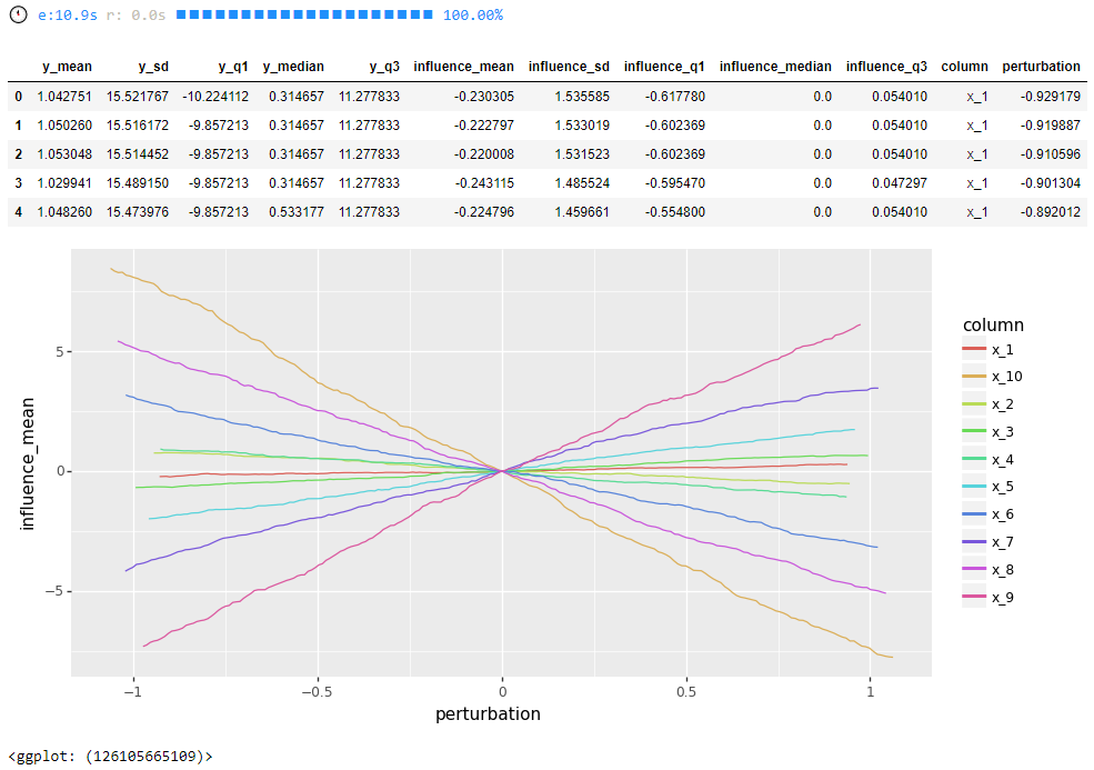
get_model_influence
from nightingale.feature_importance import get_model_influence

# import other libraries
from sklearn.ensemble import RandomForestRegressor
from sklearn.model_selection import train_test_split
from pandas import DataFrame
from numpy.random import normal
from IPython.display import display

# visualization libraries
from plotnine import ggplot, geom_line, aes, stat_smooth, facet_wrap
from plotnine.data import mtcars
from plotnine import options

# create the data
num_rows = 1000
num_columns = 10
data = DataFrame({f'x_{i + 1}': normal(size=num_rows) for i in range(num_columns)})
noise = normal(size=num_rows)
data['y'] = noise
for i in range(num_columns):
    data['y'] += data[f'x_{i + 1}'] * (i + 1) * (-1) ** i

# split the data into training and test
training, test = train_test_split(data, test_size=0.2, random_state=42)
x_columns = [f'x_{i + 1}' for i in range(num_columns)]
X_training = training[x_columns]
X_test = test[x_columns]

# build random forest regressor
random_forest_regressor = RandomForestRegressor(n_estimators=10)
random_forest_regressor.fit(X_training, training['y'])

# show results
influence = get_model_influence(model=random_forest_regressor, data=test, x_columns=x_columns, num_points=200, num_threads=1, echo=1)
display(influence.head())

# visualize
options.figure_size = 10, 5
ggplot(influence, aes(x='perturbation', y='influence_mean', colour='column')) + geom_line()
References
z-score: https://stackoverflow.com/questions/20864847/probability-to-z-score-and-vice-versa-in-python
Release history Release notifications | RSS feed


Download files
Download the file for your platform. If you're not sure which to choose, learn more about installing packages.
Source Distribution
Built Distribution
Filter files by name, interpreter, ABI, and platform.
If you're not sure about the file name format, learn more about wheel file names.
Copy a direct link to the current filters
File details
Details for the file nightingale-2020.4.7.tar.gz.
File metadata
- Download URL: nightingale-2020.4.7.tar.gz
- Upload date:
- Size: 33.1 kB
- Tags: Source
- Uploaded using Trusted Publishing? No
- Uploaded via: twine/1.12.1 pkginfo/1.4.2 requests/2.23.0 setuptools/40.8.0 requests-toolbelt/0.8.0 tqdm/4.26.0 CPython/3.7.2
File hashes
| Algorithm | Hash digest | |
|---|---|---|
| SHA256 |
c2fd5daabc1d8eccd5bd0eb1eb6e6d77480ea5bf9e279f79225f92e20b66b266
|
|
| MD5 |
decbb0654c0a010ebbb3e5ca7cc5a642
|
|
| BLAKE2b-256 |
33f853255f2db96982a1d97b727ae57c654783ec94e5f7f47c2314578c1f39ff
|
File details
Details for the file nightingale-2020.4.7-py3-none-any.whl.
File metadata
- Download URL: nightingale-2020.4.7-py3-none-any.whl
- Upload date:
- Size: 45.1 kB
- Tags: Python 3
- Uploaded using Trusted Publishing? No
- Uploaded via: twine/1.12.1 pkginfo/1.4.2 requests/2.23.0 setuptools/40.8.0 requests-toolbelt/0.8.0 tqdm/4.26.0 CPython/3.7.2
File hashes
| Algorithm | Hash digest | |
|---|---|---|
| SHA256 |
47113440b725c806d4298da40063e5e2ad4bd7e39ea1e61693c873ea52e21c76
|
|
| MD5 |
39c4a40471c9cbcbe075da30989229cd
|
|
| BLAKE2b-256 |
c82e180bb9bc2a64e0ed7a296d9acec0c6b6f8fc44f508ff2c349feca04642e1
|


