Heuristic Algorithms in Python

Project description
:clipboard: Document, :clipboard: 文档


scikit-opt
Heuristic Algorithms in Python
Genetic Algorithm, Particle Swarm Optimization, Simulated Annealing, Ant Colony Algorithm in Python
install
pip install scikit-opt
News:
All algorithms will be available on TensorFlow/Spark on version 0.4, getting parallel performance.
feature: UDF
UDF (user defined function) is available in version 0.2 release!
For example, you just worked out a new type of selection function.
Now, your selection function is like this:
def selection_elite(self):
    print('udf selection actived')
    FitV = self.FitV
    FitV = (FitV - FitV.min()) / (FitV.max() - FitV.min() + 1e-10) + 0.2
    # the worst one should still has a chance to be selected
    # the elite(defined as the best one for a generation) must survive the selection
    elite_index = np.array([FitV.argmax()])

    # do Roulette to select the next generation
    sel_prob = FitV / FitV.sum()
    roulette_index = np.random.choice(range(self.size_pop), size=self.size_pop - 1, p=sel_prob)
    sel_index = np.concatenate([elite_index, roulette_index])
    self.Chrom = self.Chrom[sel_index, :]  # next generation
    return self.Chrom
Regist your selection to GA
from sko.GA import GA, GA_TSP, ga_with_udf
options = {'selection': {'udf': selection_elite}}
GA_1 = ga_with_udf(GA, options)
Now do GA as usual
demo_func = lambda x: x[0] ** 2 + (x[1] - 0.05) ** 2 + x[2] ** 2
ga = GA_1(func=demo_func, n_dim=3, max_iter=500, lb=[-1, -10, -5], ub=[2, 10, 2])
best_x, best_y = ga.fit()

print('best_x:', best_x, '\n', 'best_y:', best_y)
Until Now, the udf surport
crossover,mutation,selection,rankingof GA
demo
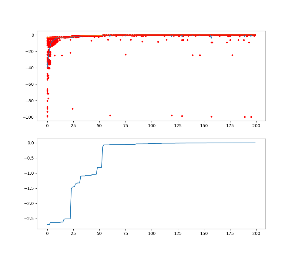
1. Genetic Algorithm
from sko.GA import GA


def demo_func(x):
    x1, x2, x3 = x
    return x1 ** 2 + (x2 - 0.05) ** 2 + x3 ** 2


ga = GA(func=demo_func, lb=[-1, -10, -5], ub=[2, 10, 2], max_iter=500)
best_x, best_y = ga.fit()
plot the result using matplotlib:
import pandas as pd
import matplotlib.pyplot as plt
Y_history = ga.all_history_Y
Y_history = pd.DataFrame(Y_history)
fig, ax = plt.subplots(3, 1)
ax[0].plot(Y_history.index, Y_history.values, '.', color='red')
plt_mean = Y_history.mean(axis=1)
plt_max = Y_history.min(axis=1)
ax[1].plot(plt_mean.index, plt_mean, label='mean')
ax[1].plot(plt_max.index, plt_max, label='min')
ax[1].set_title('mean and all Y of every generation')
ax[1].legend()

ax[2].plot(plt_max.index, plt_max.cummin())
ax[2].set_title('best fitness of every generation')
plt.show()
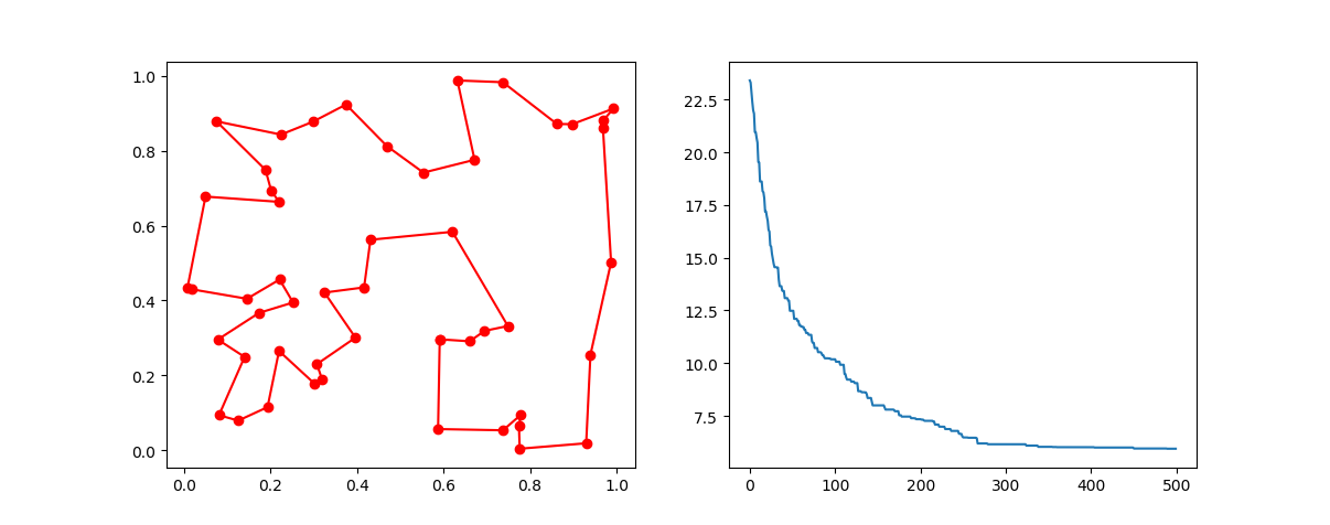
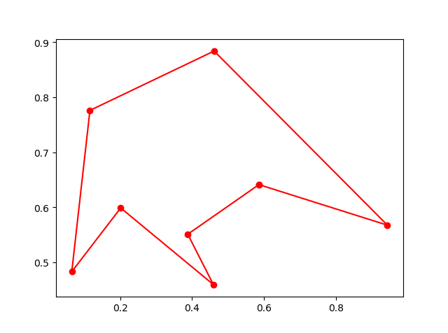
1.1 Genetic Algorithm for TSP(Travelling Salesman Problem)
Just import the GA_TSP, it overloads the crossover, mutation to solve the TSP
Firstly, your data (the distance matrix). Here I generate the data randomly as a demo:
import numpy as np

num_points = 8

points = range(num_points)
points_coordinate = np.random.rand(num_points, 2)
distance_matrix = np.zeros(shape=(num_points, num_points))
for i in range(num_points):
    for j in range(num_points):
        distance_matrix[i][j] = np.linalg.norm(points_coordinate[i] - points_coordinate[j], ord=2)
print('distance_matrix is: \n', distance_matrix)


def cal_total_distance(points):
    num_points, = points.shape
    total_distance = 0
    for i in range(num_points - 1):
        total_distance += distance_matrix[points[i], points[i + 1]]
    total_distance += distance_matrix[points[i + 1], points[0]]
    return total_distance
Do GA
from sko.GA import GA_TSP
ga_tsp = GA_TSP(func=cal_total_distance, points=points, pop=50, max_iter=200, Pm=0.001)
best_points, best_distance = ga_tsp.fit()
Plot the result:
fig, ax = plt.subplots(1, 1)
best_points_ = np.concatenate([best_points, [best_points[0]]])
best_points_coordinate = points_coordinate[best_points_, :]
ax.plot(best_points_coordinate[:, 0], best_points_coordinate[:, 1],'o-r')
plt.show()
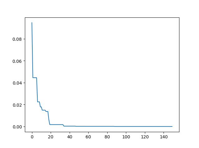
2. PSO(Particle swarm optimization)
def demo_func(x):
    x1, x2, x3 = x
    return x1 ** 2 + (x2 - 0.05) ** 2 + x3 ** 2

from sko.PSO import PSO
pso = PSO(func=demo_func, dim=3)
fitness = pso.fit()
print('best_x is ',pso.gbest_x)
print('best_y is ',pso.gbest_y)
pso.plot_history()
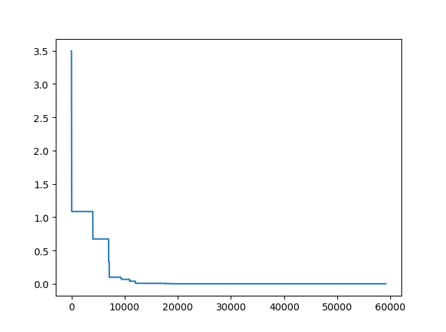
3. SA(Simulated Annealing)
def demo_func(x):
    x1, x2, x3 = x
    return x1 ** 2 + (x2 - 0.05) ** 2 + x3 ** 2

from sko.SA import SA
sa = SA(func=demo_func, x0=[1, 1, 1])
x_star, y_star = sa.fit()
print(x_star, y_star)
import matplotlib.pyplot as plt
import pandas as pd

plt.plot(pd.DataFrame(sa.f_list).cummin(axis=0))
plt.show()
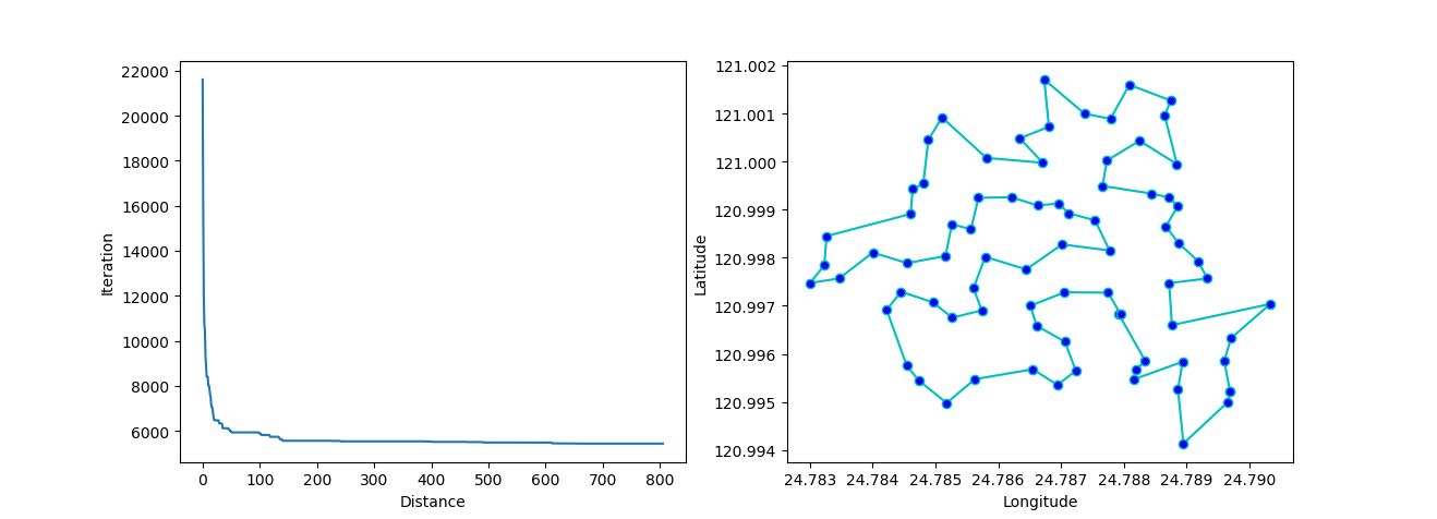
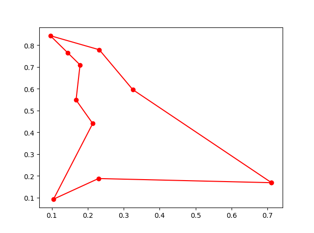
3.1 SA for TSP
Firstly, your data (the distance matrix). Here I generate the data randomly as a demo (find it in GA for TSP above)
DO SA for TSP
from sko.SA import SA_TSP
sa_tsp = SA_TSP(func=demo_func, x0=range(num_points))
best_points, best_distance = sa_tsp.fit()
plot the result
fig, ax = plt.subplots(1, 1)
best_points_ = np.concatenate([best_points, [best_points[0]]])
best_points_coordinate = points_coordinate[best_points_, :]
ax.plot(best_points_coordinate[:, 0], best_points_coordinate[:, 1], 'o-r')
plt.show()
4. ASA for tsp (Ant Colony Algorithm)
aca = ACA_TSP(func=cal_total_distance, n_dim=8,
              size_pop=10, max_iter=20,
              distance_matrix=distance_matrix)

best_x, best_y = aca.fit()
5. immune algorithm (IA)
from sko.IA import IA_TSP_g as IA_TSP

ia_tsp = IA_TSP(func=cal_total_distance, n_dim=num_points, pop=500, max_iter=2000, Pm=0.2,
                T=0.7, alpha=0.95)
best_points, best_distance = ia_tsp.fit()
print('best routine:', best_points, 'best_distance:', best_distance)
6. artificial fish swarm algorithm (AFSA)
def func(x):
    x1, x2 = x
    return 1 / x1 ** 2 + x1 ** 2 + 1 / x2 ** 2 + x2 ** 2


from sko.ASFA import ASFA

asfa = ASFA(func, n_dim=2, size_pop=50, max_iter=300,
            max_try_num=100, step=0.5, visual=0.3,
            q=0.98, delta=0.5)
best_x, best_y = asfa.fit()
print(best_x, best_y)
Release history Release notifications | RSS feed


Download files
Download the file for your platform. If you're not sure which to choose, learn more about installing packages.
Source Distributions
Built Distribution
Filter files by name, interpreter, ABI, and platform.
If you're not sure about the file name format, learn more about wheel file names.
Copy a direct link to the current filters
File details
Details for the file scikit_opt-0.3.1-py3-none-any.whl.
File metadata
- Download URL: scikit_opt-0.3.1-py3-none-any.whl
- Upload date:
- Size: 16.4 kB
- Tags: Python 3
- Uploaded using Trusted Publishing? No
- Uploaded via: twine/1.13.0 pkginfo/1.5.0.1 requests/2.21.0 setuptools/40.8.0 requests-toolbelt/0.9.1 tqdm/4.31.1 CPython/3.7.1
File hashes
| Algorithm | Hash digest | |
|---|---|---|
| SHA256 |
1963adaf43b0a42d233c2020d21ab32566f895e674e275189599e0b0a2a1c2f4
|
|
| MD5 |
5364c78c07bf56255b97244ff3b2e6cd
|
|
| BLAKE2b-256 |
0270d345818f77cfe310ea937267b06ed98a8c7912a9eb4edc28db349fcae54b
|


