tsforecasting 1.2.92

TSForecasting is an Automated Time Series Forecasting Framework

TSForecasting - Automated Time Series Forecasting Framework

Framework Contextualization

The TSForecasting project offers a comprehensive and integrated pipeline designed to Automate Time Series Forecasting applications. By implementing multivariate approaches that incorporate multiple regression models, it combines multiple relevant modules such as SKLearn, AutoGluon, CatBoost and XGBoost, following an Expanding Window structured approach for performance evaluation ensuring a robust, scalable and optimized forecasting solution.

The architecture design includes five main sections, these being: data preprocessing, feature engineering, hyperparameter optimization, forecast ensembling and forecasting method selection which are organized and customizable in a pipeline structure.

This project aims at providing the following application capabilities:

• General applicability on tabular datasets: The developed forecasting procedures are applicable on any data table associated with any Time Series Forecasting scopes.

• Hyperparameter optimization and customization: It provides full configuration for each model hyperparameter through the customization of model_configurations dictionary, allowing optimal performance to be obtained for any use case.

• Robustness and improvement of predictive results: The implementation of the TSForecasting pipeline aims to improve the predictive performance directly associated with the application of the best performing forecasting method.

Main Development Tools

Major frameworks used to built this project:

• Sklearn
• AutoGluon
• CatBoost
• XGBoost
• LightGBM

Performance Evaluation Structure

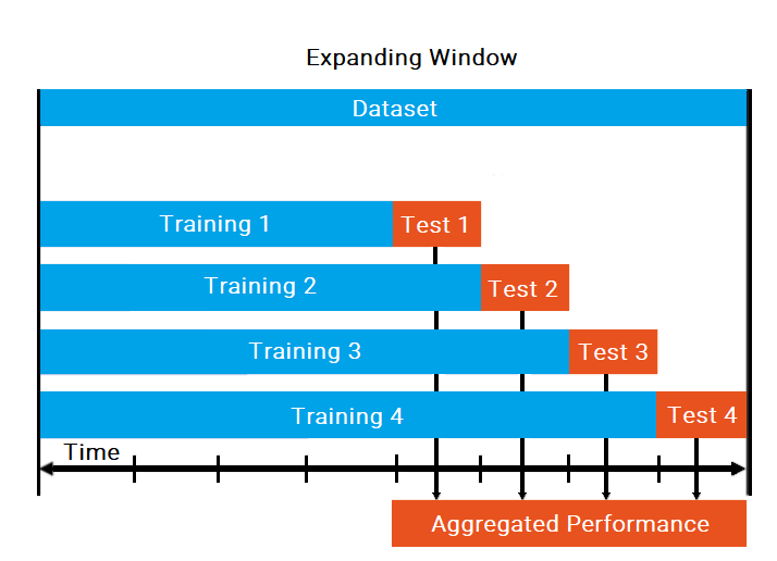
The Expanding Window evaluation technique is a temporary approximation on the real value of the time series data. The first test segment is selected according to the train length and then it's forecasted in accordance with forecast size. The starting position of the subsequent segment is set in direct relation to the sliding window size, this meaning, if the sliding size is equal to the forecast size, each next segment starts at the end of the previous. This process is repeated until all time series data gets segmented and it uses all the iterations and observations to construct an aggregated and robust performance analysis to each predicted point.

Where to get it

The source code is currently hosted on GitHub at: https://github.com/TsLu1s/TSForecasting

Binary installer for the latest released version is available at the Python Package Index (PyPI).

Installation

To install this package from Pypi repository run the following command:

pip install tsforecasting

Usage Examples

1. TSForecasting - Automated Time Series Forecasting

The first needed step after importing the package is to load a dataset and define your DataTime (datetime64[ns] type) and Target column to be predicted, then rename them to Date and y, respectively. The following step is to define your future running pipeline parameters variables, these being:

• train_size: Length of Train data in which will be applied the first Expanding Window iteration;

• lags: The number of time steps in each window, indicating how many past observations each input sample includes;

• horizon: Full length of test/future ahead predictions;

• sliding_size: Length of sliding window, sliding_size>=horizon is suggested;

• models: All selected models intented to be ensembled for evaluation. To fit and compare predictive performance of available models set them in paramater models:list, options are the following:

  • RandomForest
  • ExtraTrees
  • GBR
  • KNN
  • GeneralizedLR
  • XGBoost
  • LightGBM
  • Catboost
  • AutoGluon

• hparameters: Nested dictionary in which are contained all models and specific hyperparameters configurations. Feel free to customize each model as you see fit (customization example shown bellow);

• granularity: Valid interval of periods correlated to data -> 1m,30m,1h,1d,1wk,1mo (default='1d');

• metric: Default predictive evaluation metric is MAE (Mean Absolute Error), other options are MAPE (Mean Absolute Percentage Error) and MSE (Mean Squared Error);

The fit_forecast method set the default parameters for fitting and comparison of all segmented windows for each selected and configurated model. After implementation, the history method agregates the returning the variable fit_performance containing the detailed measures of each window iteration forecasted value and all segmented iterations performance.

The forecast method forecasts the future values based on the previously predefined best performing model.

from tsforecasting.forecasting import (TSForecasting,
                                       model_configurations)
import pandas as pd
import warnings
warnings.filterwarnings("ignore", category=Warning) #-> For a clean console

## Dataframe Loading
data = pd.read_csv('csv_directory_path') 
data = data.rename(columns={'DateTime_Column': 'Date','Target_Name_Column':'y'})
data = data[['Date',"y"]]
    
## Get Models Hyperparameters Configurations
parameters = model_configurations()
print(parameters)

# Customization Hyperparameters Example
hparameters["RandomForest"]["n_estimators"] = 50
hparameters["KNN"]["n_neighbors"] = 5
hparameters["Catboost"]["iterations"] = 150
hparameters["AutoGluon"]["time_limit"] = 50

## Fit Forecasting Evaluation
tsf = TSForecasting(train_size = 0.90,
                    lags = 10,
                    horizon = 10,
                    sliding_size = 30,
                    models = ['RandomForest', 'ExtraTrees', 'GBR', 'KNN', 'GeneralizedLR',
                              'XGBoost', 'LightGBM', 'Catboost', 'AutoGluon'],
                    hparameters = hparameters,
                    granularity = '1h',
                    metric = 'MAE'
                    )
tsf = tsf.fit_forecast(dataset = data)

# Get Fit History
fit_performance = tsf.history()

## Forecast
forecast = tsf.forecast()

2. TSForecasting - Extra Auxiliar Methods

The make_timeseries method transforms a DataFrame into a format ready for time series analysis. This transformation prepares data sets for forecasting future values based on historical data, optimizing the input for subsequent model training and analysis, taking into consideration both the recency of data and the horizon of the prediction.

• window_size: Determinates how many past observations each sample in the DataFrame should include. This creates a basis for learning from historical data.
• horizon: Defines the number of future time steps to forecast. This addition provides direct targets for prediction models.
• granularity: Adjusts the temporal detail from minutes to months, making the method suitable for diverse time series datasets (options -> 1m,30m,1h,1d,1wk,1mo).
• datetime_engineering: When activated enriches the dataset with extra date-time features, such as year, month, and day of the week, potentialy enhancing the predictive capabilities of the model.

from tsforecasting.forecasting import Processing

pr = Processing()

data = pr.make_timeseries(dataset = data,
			  window_size = 10, 
			  horizon = 2, 
			  granularity = '1h',
			  datetime_engineering = True)

License

Distributed under the MIT License. See LICENSE for more information.

Contact

Luis Santos - LinkedIn